Balance I: How to measure Understeer and Oversteer
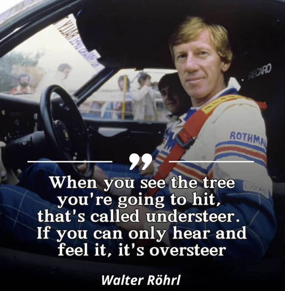
Engineers and manufacturers are constantly searching for ways to extract more grip from a vehicle. However, there is another characteristic that drivers often perceive even more clearly than absolute grip itself: vehicle balance.
Whether it is a professional driver operating at the limit in motorsport or a road driver during everyday use, balance largely determines how predictable and confidence-inspiring a vehicle feels.
An incorrect balance can manifest itself in two opposite ways. The vehicle may feel reluctant to rotate, forcing the driver to apply excessive steering input to negotiate a corner, or it may feel unstable and nervous, giving the impression that it could rotate uncontrollably at any moment. Both situations are a consequence of an improper distribution of available grip between the front and rear axles.
To quantify these behaviours, we first define an ideal steering angle for any given cornering condition. This reference value will be referred to as the neutral steering angle and will be compared with the real steering wheel position to quantify the level of undesteer or oversteer a car has.
Neutral Steering
The concept is straightforward. If the steering angle required to negotiate a corner is greater than the neutral steering angle, the vehicle is considered to exhibit understeer. In this case, the front axle generates less lateral capability than the rear axle and therefore requires additional steering input to achieve the desired cornering radius.
Conversely, if the required steering angle is smaller than the neutral steering angle, the vehicle exhibits oversteer, indicating that the rear axle is limiting the vehicle's cornering performance.
The figure below compares the calculated neutral steering channel in red with the actual steering input in yellow recorded during a lap of the Barcelona circuit.
By comparing the neutral steering angle with the measured steering angle, we obtain a new channel referred to as the balance channel.
Positive values indicate understeer, while negative values indicate oversteer.
The balance channel is shown in the lower section of the plot in green.
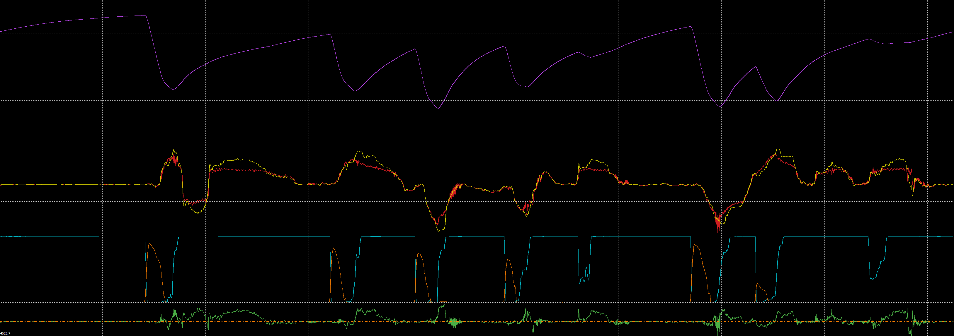
In this particular example, the vehicle exhibits a predominantly understeering behaviour, as the actual steering angle remains above the neutral steering angle for most of the lap. While this qualitative assessment is useful, a proper engineering analysis requires objective metrics capable of summarising the behaviour numerically. This is why we use what we call metrics, which help us to understand the balance of our vehicle just with a number.
Metrics
The first ( and very primitive ) metric consists of averaging the balance channel over an entire lap.
In the example we are using this metric gives as an output a value of 3.99
This provides a single numerical value representing the overall balance characteristic of the vehicle.
However, this metric has an important limitation.
Imagine a situation where the car exhibits severe understeer in half of the corners and severe oversteer in the other half. The positive and negative contributions could cancel each other out, resulting in an overall balance value close to zero. The metric would suggest a neutral vehicle, despite the fact that the car would be extremely difficult to drive.
To overcome this limitation, the balance metric should also be evaluated on a corner-by-corner basis or at least in function of the corner characteristics. The most extended way to use the balance metric in race engineering is to separate corners into high, medium and low speed.
This approach provides a much more representative picture of the vehicle's behaviour around the circuit.
In this particular case we can observe that the faster the corner is the more understeer behaviour the vehicle presents.
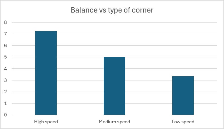
At high speeds, aerodynamic balance has a dominant influence on vehicle behaviour. At low speeds, where aerodynamic loads are significantly reduced, mechanical balance becomes the primary contributor.
For trackside analysis, separating the balance metric into high-speed, medium-speed and low-speed corner groups can provide valuable guidance when evaluating setup changes and help avoid misleading conclusions.
Corner Phase Analysis
A further level of refinement can be achieved by separating each corner into individual phases.
For the purpose of this analysis, the corner will be divided into three sections:
- Corner Entry
- Mid-Corner
- Corner Exit
Corner entry begins when the driver applies brake pressure and ends when braking is significantly reduced while a meaningful steering input is already present.
The mid-corner phase corresponds to the period where the vehicle is predominantly coasting. Driver inputs are minimal, steering angle typically reaches its maximum value, and peak lateral acceleration is usually achieved.
Corner exit begins when throttle application starts and ends once the vehicle is fully accelerated and has completed the corner.
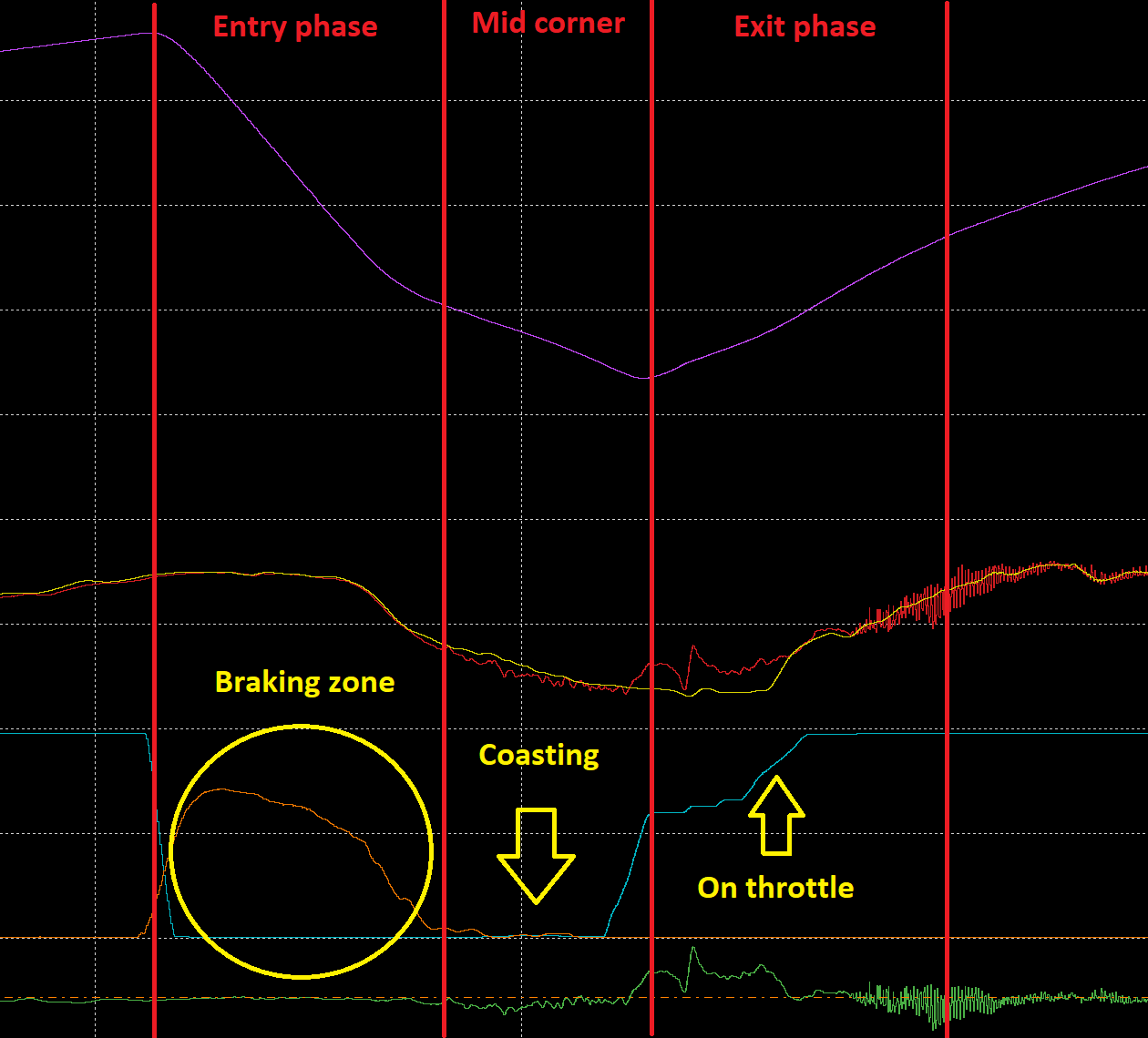
Vehicle balance does not necessarily remain constant throughout these phases. A car may exhibit understeer on entry while becoming oversteer-limited on exit, or vice versa, like in the example shown below.
By calculating the balance metric independently for each phase, these behaviours can be quantified and visualised.
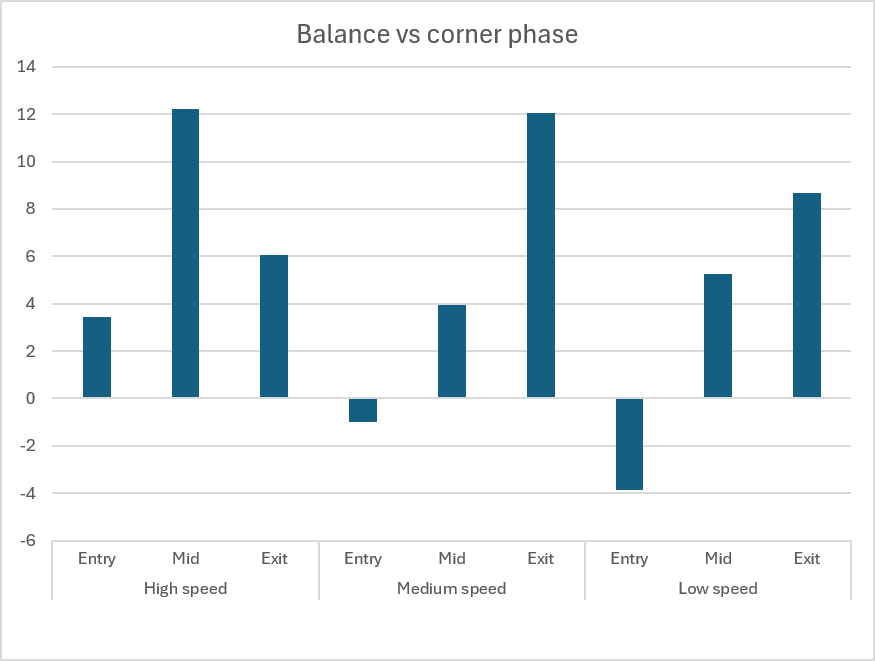
In the example above, we can easily spot how our biggest balance issues are mid corner understeer in fast corners, and exit understeer in medium speed corners.
This level of detail greatly improves the quality of setup decisions. For instance, we are going to try an increase in front wing angle of 1.5 degrees without compensating our ride heights, around a 2% of aerobalance moved forward, to evaluate the impact of the change. In theory, this change should impact high speed corners the most, having little impact in low speed corners.
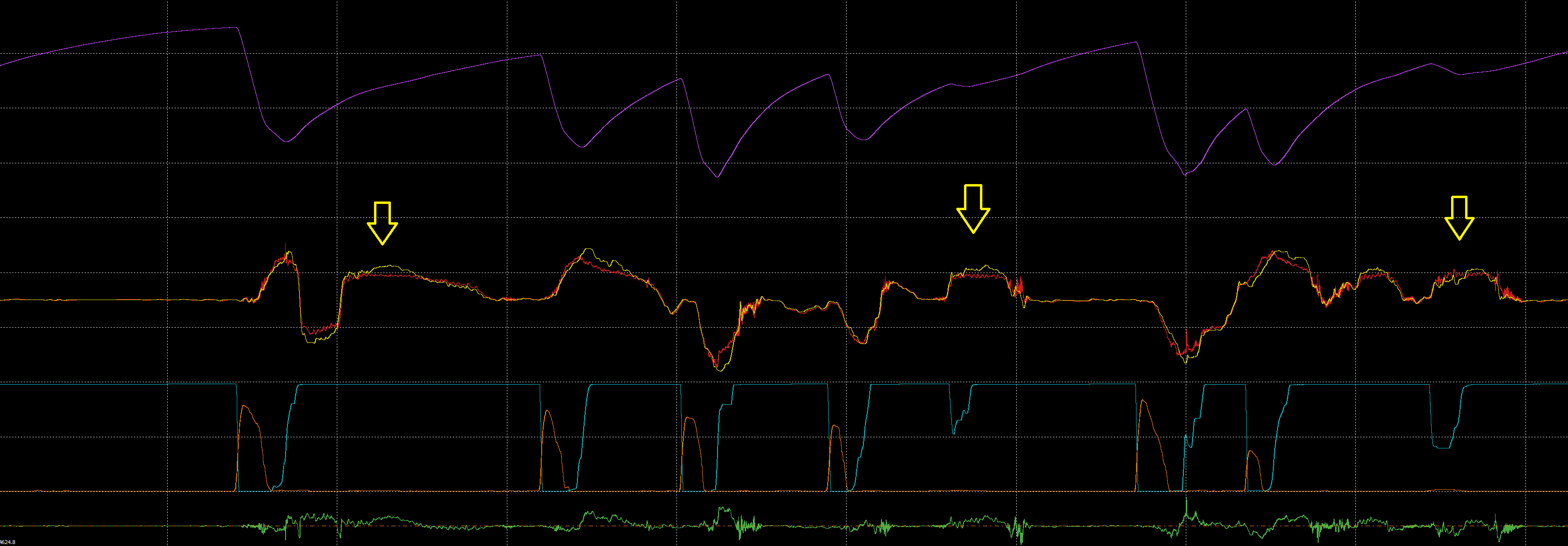
In the time/distance graph from above it can already be seen how the understeer has been reduced in the fast corners. But as stated earlier, to do proper engineering we need to give numbers to it to know by how much.
The metrics show the following:
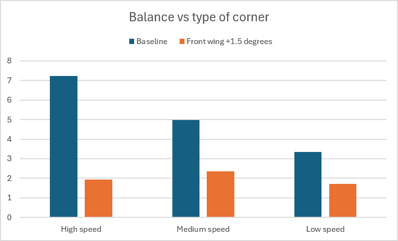
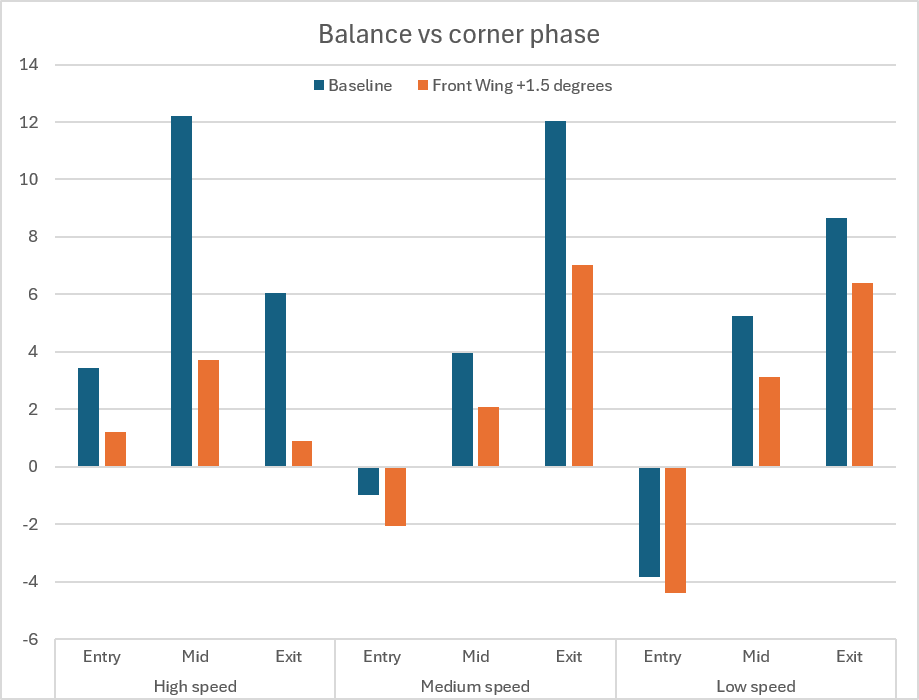
The results show a reduction of 5 points in high speed corners, mainly in the mid corner phase, the one we wanted t0 fix.
After this test, we can state that a change of 2% in aero balance resulted in 5 points less in the balance metric, and as a consequence the next time we see a balance issue, we will be able to decide how big of a change we need to do to fix an unwanted balance.
This was a very basic example of how to quantify a car’s balance, but the real key is determining how to set the reference for the neutral steer angle. This is where things get a bit more numerical—and trickier.
If you’re interested in this topic, follow us. We’ll explain in detail how to calculate the “Neutral Steer Angle” channel and why the definition of balance provided by Milliken cannot be directly applied to motorsport applications.
Liked this article? Check the previous one!
 Antonio Ortiz Poveda